
08 Jul Index Match Excel Lookup
Howdee folks! VLOOKUP is a great Excel function, but sometimes you need a little more flexibility than it provides. That’s where nesting the MATCH formula inside the INDEX (also known as the index match excel function) formula can shine. It also has the added benefit of impressing the heck out of people who don’t know about it! Let’s say you have some data like we see here…

…and the user wants to be able to select accounts and months for comparison. You can use the INDEX MATCH Excel functions to make this very interactive for the user. So – let’s divert from the problem for a moment and learn what exactly the INDEX and MATCH formulas are.
What is the INDEX function?
Syntax: INDEX(array,row_num,column_num)
The INDEX function, simply put, is a means to return data from a cell based on its coordinates within an array (in this case, the array is a two-dimensional array, or table). Imagine a tic-tac-toe board as an Excel spreadsheet in cells A1 to C3 like you see below.

If you wanted to place an “X” in the center using the INDEX function, you would reference the coordinates (2,2). In the formula this would look like INDEX(A1:C3,2,2). The first 2 references the row number, and the second 2 references the column number. Therefore (1,2) would reference the first row and second column.
What is the MATCH function?
Syntax: MATCH(lookup_value,lookup_array,match_type)
Now that we know what the INDEX function is, let’s explore the MATCH function. The MATCH function returns the position of a certain item in a one-dimensional array (or list). What does this mean? Let’s say we have a list of names in Excel starting in cell A1 and we want to determine the position of one of those names in the list. The MATCH function can help us like so:

You can see that the result of the formula tells us that “Ryan” is in position 4 of this one-dimensional array (list). Note that the last input of the formula is “match_type”. This is mostly going to be 0 in the context of this article. You might use the 1 and -1 inputs if you’re finding the positions of numbers in a list.
Index Match Excel Function
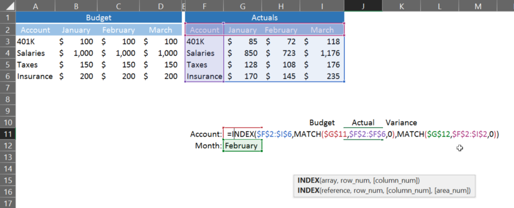
Now – back to our problem of creating an interactive report for our user. We can combine the INDEX MATCH Excel functions using inputs from the user to define the coordinates we need to select. See below:
Our user now has the ability to select his/her inputs! Here are the formulas driving this functionality.
The Formulas:

I hope this trick is as helpful to you as it has been to me over the years. I use this when I need to give the end user flexibility to select inputs or when data isn’t always organized the same so VLOOKUP isn’t as effective.
One important note is that your INDEX Array should include any potential rows/columns your user may need to reference. Also, your MATCH arrays need to the same size as the length and width of your INDEX array, otherwise you will get an error because Excel will not be able to compare the arrays correctly. Lastly, the MATCH arrays do not need to always be the leftmost column and top row of your INDEX array. If they’re the same length/width as the INDEX array, you can place them anywhere within your data. Super helpful if you’re going to be dropping in an export to this tool every so often.
Please let me know if this was helpful to you or, if you have questions, drop those in the comments!
Cheers!
R
No Comments