Everything You Need to Know About Creating a Dropdown in Excel

31 Jul Everything You Need to Know About Creating a Dropdown in Excel

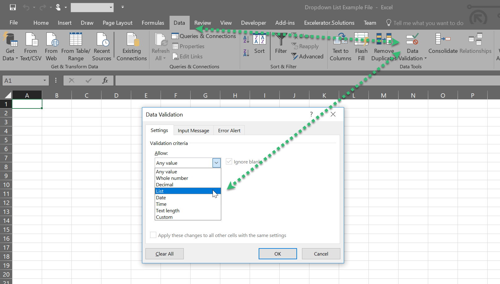
Howdee! There will be occasions, when working with Microsoft Excel, when you want to control the data that can be entered in a certain cell. A great way to accomplish this is creating a dropdown in Excel that the end user can select values from. This is achieved by using data validation to create a dropdown list in a cell, as shown here.

There are a handful of different ways to populate the list and, depending on the situation, they can all be viable options. You can create a dropdown in Excel that is hard-coded into the data validation rule, it can reference a range of data, a table of data, or even be defined by using formulas. We will cover off on each of these individually in this article and discuss some pros & cons I’ve discovered over the years.

Hard-coding a Dropdown in Excel

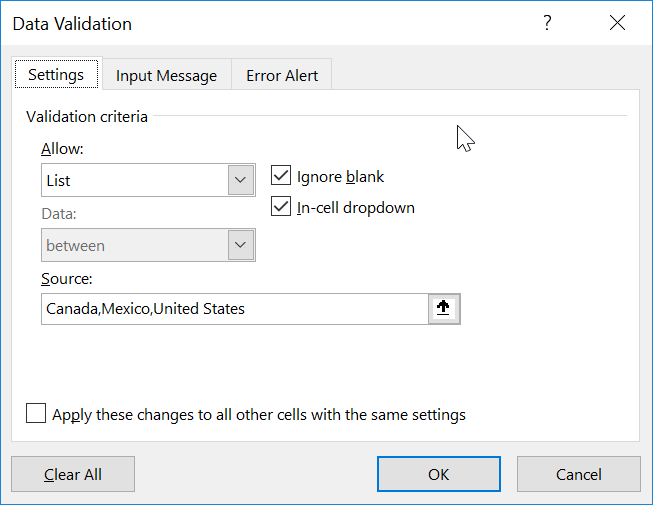
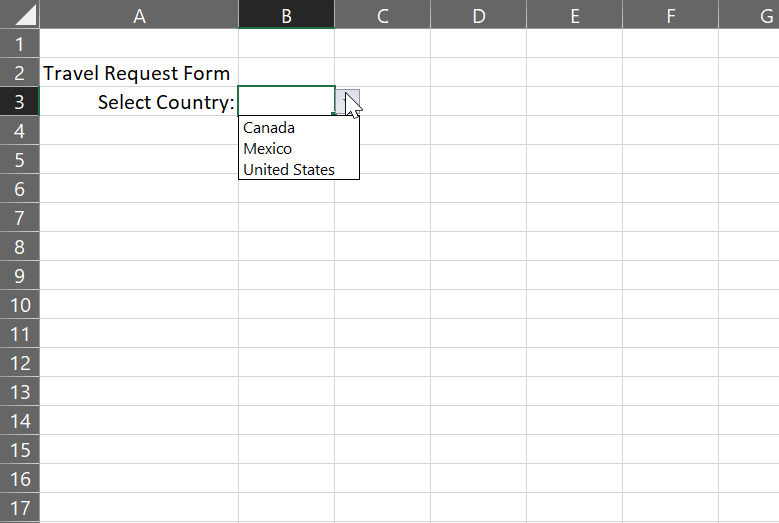
The simplest method to make a dropdown in Excel is to simply hard-code your list into the data validation rule.  Let’s assume we were creating a travel request form and wanted to have a dropdown list of countries to select from. Using this technique, we’d just type the country names in separated by commas as shown in the screen grab. The result is a dropdown that is populated with Canada, Mexico, and United States.

This method is useful for short Excel dropdowns that aren’t going to change very often (or ever). It does not require any of the information to be populated in a hidden sheet that a user could potentially unlock and edit so is slightly more secure. However, it is not practical for longer lists, lists that could change regularly, or lists that need to be more dynamic in nature. I generally use this method for “this or that” type lists where the user is only selecting from one of two options.

Creating a Dropdown by Referencing a Range of Cells

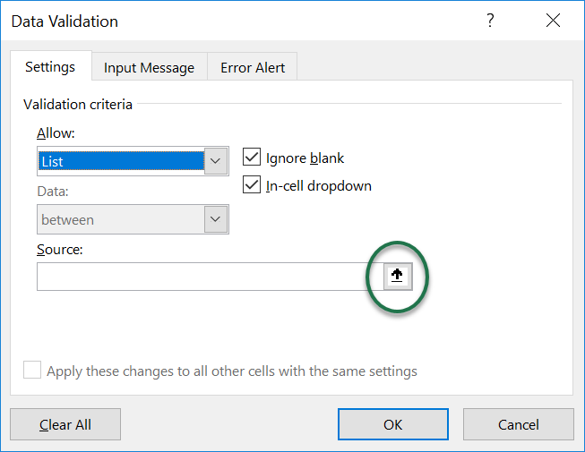
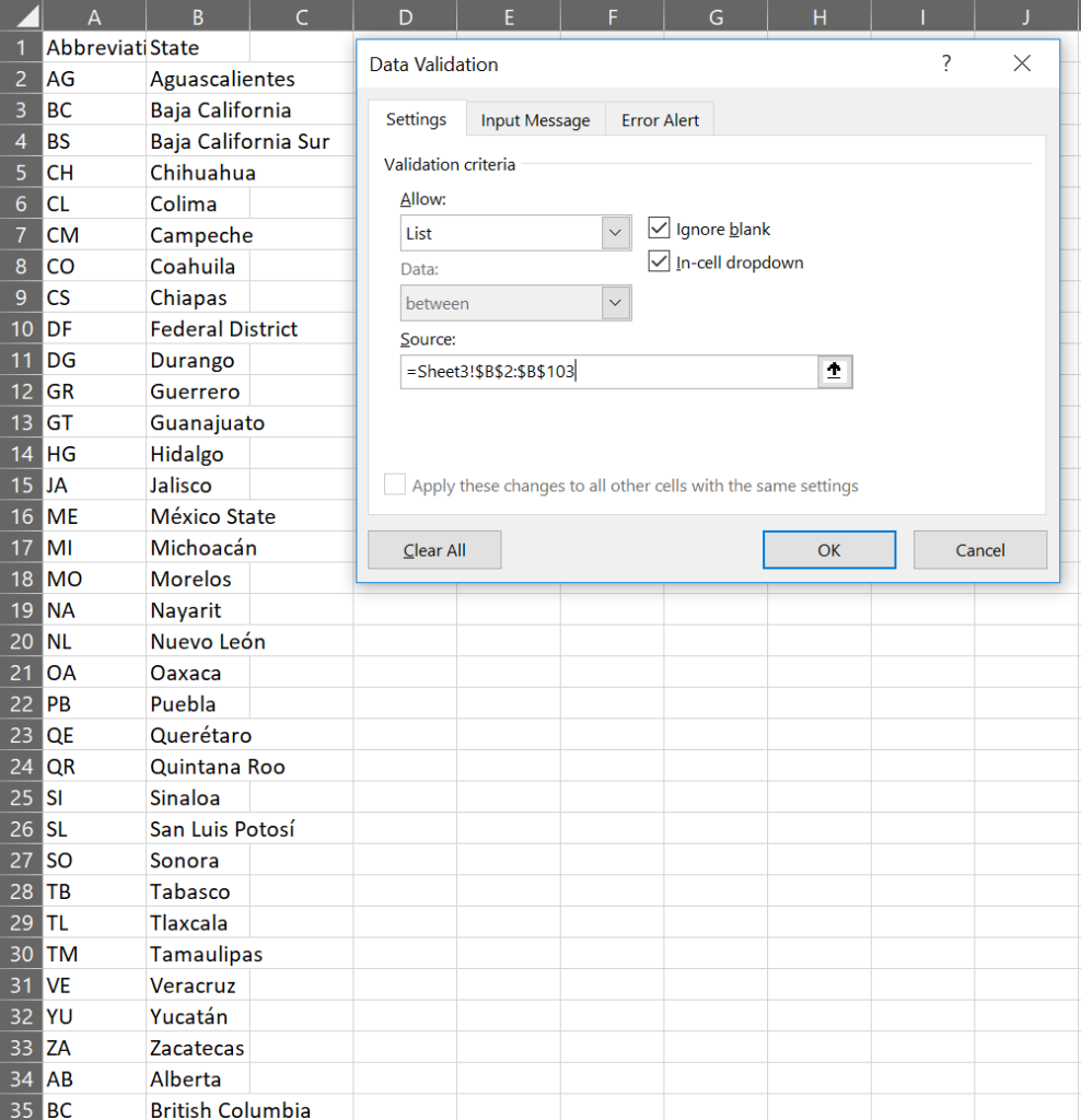
If you have a list that is a bit longer or needs to be updated regularly, it is generally easier to input the information in a separate sheet and then reference it from the data validation interface. For instance, if we want the user to be able to select a state, we could create a separate sheet with list of possible states and reference those lists. To do that, click the underlined-up arrow (highlighted in screen grab below) in the data validation window, and then select your range. If you’re more comfortable typing in the range reference, you can do that as well.

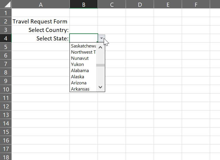
As you can see, we’ve created a dropdown in Excel by referencing the ranges in which the data is stored. This saved a significant amount of time over typing in the list of states separated by a comma. However, this dropdown is very long and contains all states from the three countries in our first dropdown. This is the primary issue with simply selecting a range of data. To separate the lists by state, we’d have to select three dropdowns in this fashion. This is not efficient and is definitely not great for user experience (something you should always keep in mind when building templates). However, by using functions in our data validation source, we can make this dropdown list dependent on the value selected in the country dropdown. That brings us to…

Creating a Dependent Dropdown in Excel

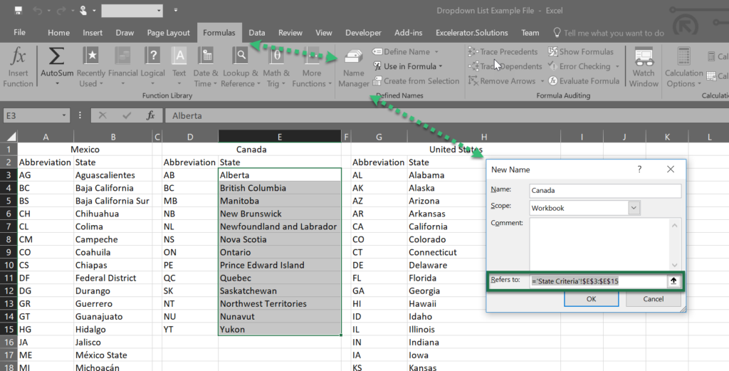
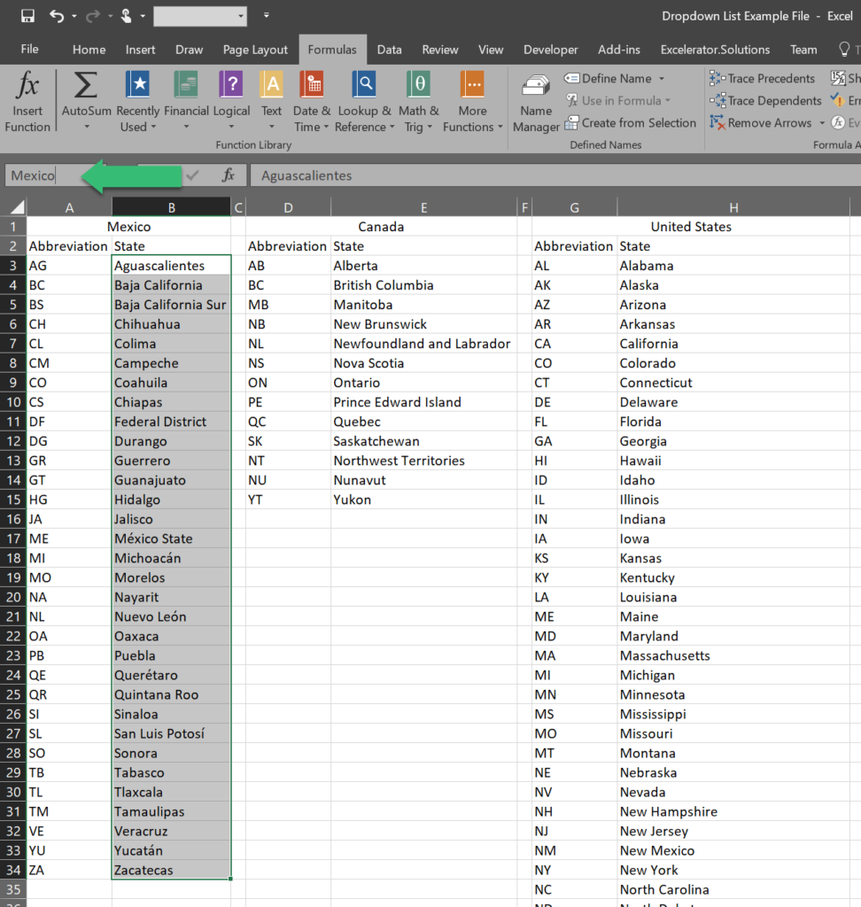
Creating a dependent dropdown in Excel is great from both an efficiency and user experience perspective. It requires a little extra effort at setup but is easy to maintain in the long run. For this approach, you’ll need to separate your data out so it’s easy to identify what belongs where. For this example, I’ve broken out the state lists by country. From here, we will want to name the range of cells that contain the states for each country. Be sure you only select the states and not the header as whatever you select will show up in your dropdown. There are two ways to name a range in Excel. You can highlight the range you wish to name and type the name in the “Name Box” to the left of the formula bar, or you can use the “Name Manager” on the Formulas ribbon tab. I’ve shown an example of both in screen grabs below.

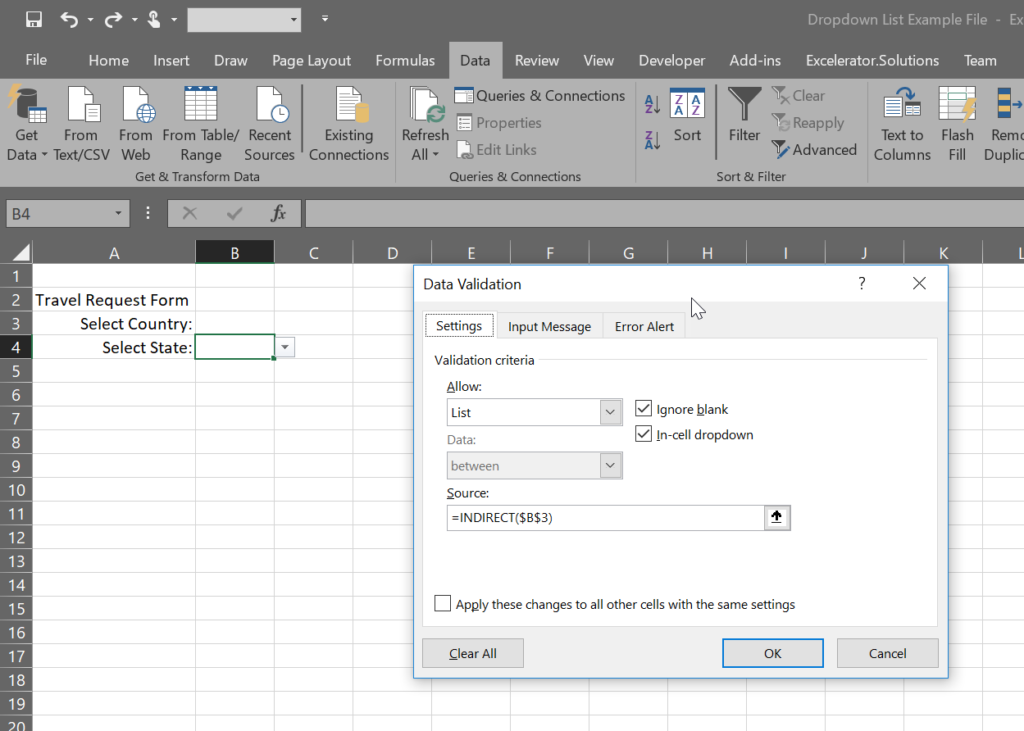
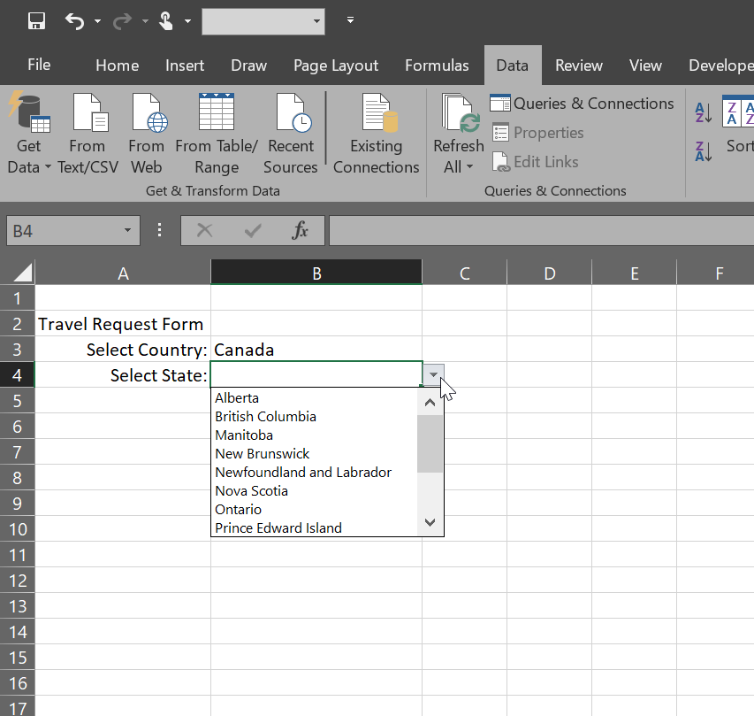
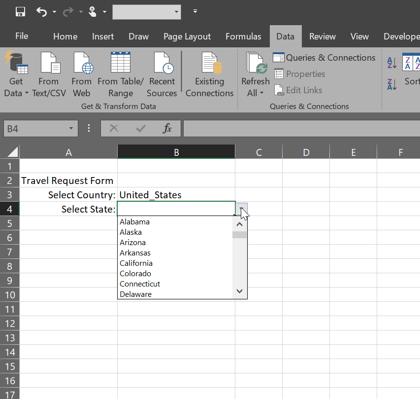
I’ve named the ranges after the values in my original dropdown. This was done on purpose to simplify step two. For this step, we will be utilizing the INDIRECT function. The indirect function returns a reference based on a text string you enter. If you use the indirect function in conjunction with your named ranged, it will return a reference to the range. This way, by using the initial dropdown as the input for our indirect function (shown below in screen grab), we have created a dynamic dropdown in Excel that will change based on what’s selected in the first.

The end user can now change countries and the list will automatically change based on their input from the first dropdown. Creating a dropdown in Excel like this will keep your templates organized and make the end user’s experience much more enjoyable. Still, this approach is not without its disadvantages. If the list is ever extended or condensed, you will have to go back to the name manager and change the size of your named range or you could be missing data or have blank selections in your dropdown. You could always ensure you insert a row into the middle of a named range but that isn’t practical if you ever hand this off to someone who isn’t aware of this. To make this even easier, let’s use tables to create our dropdown in Excel.

Using Tables as References for Dropdown Lists

The process for using tables as references for your list data is very like the process we went through for using named ranges. The indirect function is still used in our data validation source to reference data. However, you’ll be referencing the name of the table instead of the name of the range. In this example, I’ve removed the named ranges and replaced them with tables with the same names. However, there is one additional step needed in our formula. We must instruct the dropdown which table column to return. Otherwise, it will return every value in the table. This is as simple as concatenating the table name in brackets as shown here.

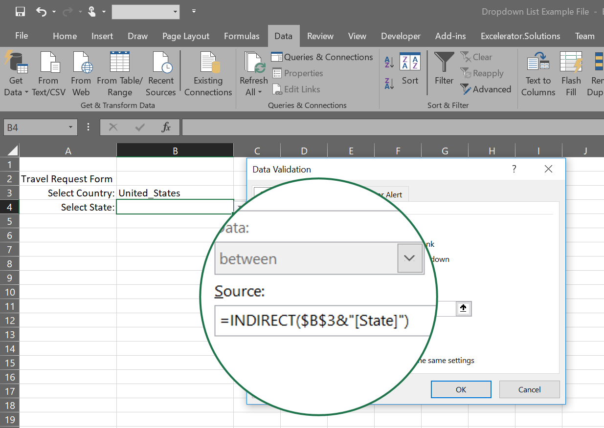
After this, the functionality is the same as the previous example. The upside here is, as long as you append/remove values to/from that table, your dropdown will always include new rows and remove deleted rows without having to change anything about the reference. If you’re a free member, feel free to download the example file here and play around with this. This practice makes managing your dropdown in Excel a breeze and, you can now let someone other than yourself manage this file and you’re not at risk of them breaking the functionality of the spreadsheet.

You should now be adequately equipped to create your own dropdown in Excel. If you have other tips on dropdowns, or have any questions about the methods above, please drop them in the comments below.

Cheers!

R