Creating Dynamic Ranges & Inputs Using the Excel Offset Function

21 Aug Creating Dynamic Ranges & Inputs Using the Excel Offset Function

Howdee! One of my favorite data analysis tools is the offset Excel function. It provides a tremendous amount of flexibility to automate ranges and formula inputs. It can be used to adjust inputs based on counts, dates, & amounts. Imagine a sum formula that automatically resizes itself to include all relevant data in a data set without needing any updates form you? This, and much more, is possible using the Excel offset function.

Excel Offset Function Syntax

Firstly, I want to cover off on the syntax of the offset Excel function. Even for advanced users, this formula can be awkward to use until you’re used to it. But, before that, someone new to the offset function might ask “what the heck does it do?”. In Excel terms, it returns a reference to a range that is a certain number of rows and columns away from a designated reference. That’s a bit difficult to digest without a visual aid so let’s use one. Imagine the below grid as a range of cells in Excel.

The offset Excel function accepts a reference point as its first input. In this grid, that would be (0,0). From there you can command to select a single cell, or a range of cells, by instructing the function to move a certain number of rows/columns away. Let’s explore the syntax and hopefully this will make more sense.

Syntax : =OFFSET(reference,rows,cols,height,width)

• Reference: This is the initial reference point from which you will instruct the function to move away from this point based on a certain logic. In the grid above, this is (0,0).
• Rows: This input will instruct the function to move a given number of rows away from the reference point. If we input a 2, the reference will point two rows down, or the third row in the example above.
• Cols: This input is the exact same as the rows input, but drives the column selection. If we also put a 2 here, the function will be pointing to the third row and third column (denoted by (2,2) in the grid above).
• Height: This input tells the function the row size of the end range to select. If you’re selecting a single cell, this will be 1. A “2” would result in two rows being selected in the final range.
• Width: This input tells the function the columns size of the end range to select. Like “Height”, if you’re selecting a single cell, the input is 1. If you’re selecting a larger range, the input would be larger.

Now, using our grid example, let’s say coordinates (0,0) is Cell A1 in Excel. The Excel offset function syntax to select (2,2) only would be =OFFSET(A1,2,2,1,1). If you wanted to select the range containing coordinates (2,2), (2,3), (3,2), & (3,3), that formula would be =OFFSET(A1,2,2,2,2). Now you’re reference encompasses all four cells in that range. If you’re struggling to understand the practical application of this, that’s ok. I did not either when someone introduced me to the formula. Let’s discuss a few uses of the function now.

Excel Offset Function for Dynamic Sum Formulas

If you create any kind of monthly report, you’ve probably had to ensure all your sum formulas included the new data you imported. It’s a tedious task on larger reports that have complex formats. However, if we use the offset Excel function to dynamically resize our sum formula input, we can effectively automate this process. Let’s assume we have a small report like the one pictured below:

If we want to populate a budget vs. actual report, we would have to resize our formulas each month when we input new data unless we can dynamically update the range when new data is entered. That’s exactly what the offset function allows us to do. See it in action here:

As you can see, the input of new data drives the size of both the quarter to date actuals and quarter to date budget. Those respective formulas for the sales line are:

Actuals : =SUM(OFFSET($A3,0,1,1,COUNTA($B3:$D3)))

Budget : =SUM(OFFSET($A3,0,5,1,COUNTA($B3:$D3)))

The only difference is the number of columns we are moving the range to the right. Otherwise, they’re the exact same. I’m using the COUNTA formula (which counts all non-blank items) to tell my offset function how wide my sum formula should be. There are other ways to resize your range as well. Any other Excel formula that returns a number result will work (MONTH, MATCH, COUNTBLANK, etc.).

Using Offset Excel Function to Dynamically Populate Dropdowns

Creating dropdowns in Excel is a terrific way to ensure data accuracy on templates. However, updating the dropdown lists can become a bit tedious. It requires not only additional data entry, but often requires resizing the range to which your dropdown is pointing. That’s where using the offset Excel function can really help. By the way, if you need a crash course on dropdowns, consider reading my blog post on dropdowns.

Let’s assume we have a list of names that populates a dropdown list of employees for a report. We would likely have employees coming to and leaving the organization and might need to have that dropdown adjusted on a regular basis. Using an offset function in the data validation window, can help us with this.

Now, as we add names to the list in column A, the dropdown in cell D3 will automatically update to include the newly added employee(s). Using the offset Excel function in this way can be a huge time saver when you have dozens of dropdowns to update.

Using Excel Offset Function to Dynamically set Database Formula Criteria (Advanced)

This is my favorite use of the offset function. It’s a tremendous help when performing analysis on large datasets. I’ll be demoing it with the DCOUNT & DSUM functions today, but you can use it with any database function. To learn about the DCOUNT function, check out the support page here (there is a similar page for DSUM). At a high level, the DCOUNT function will count unique records based on criteria I provide, while the DSUM will do the same but sum instead of count. I have some data from www.nyc.gov about job openings and want to gather information about the number of jobs based on certain criteria.

Before we start using the Excel offset function to return results, we need to set up our criteria. This will take some time when you’re new to using this approach, but it gets significantly easier the more you do it. First, let’s examine a sample of our data:

In this example data set, I’ve chosen to allow the end user to count different openings and sum the total number of openings based on the Agency, Posting Type, and Civil Service Title. In order to accomplish this, I’ve created a separate “Criteria” tab. This includes a distinct list of each of the three columns I specified. Next, the ranges need to be named so we can reference them in future steps. We will name the data in each column after the column header, like so:

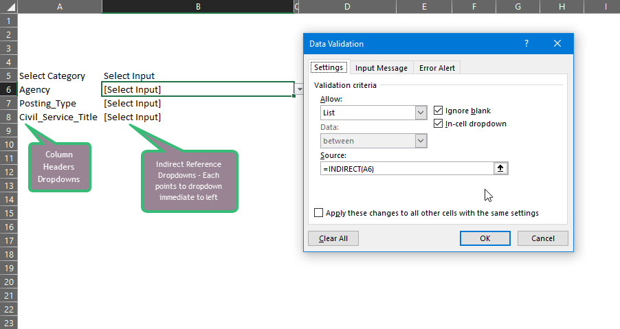
Now, after this is complete, let’s create a separate tab for the user to interact. On this tab, we will create six drop downs. Three of the dropdowns will be the exact same. They will reference the column headers (that also reference the title of the ranges we just created). The next three dropdowns will reference a separate instance of the first dropdown using the indirect function. That looks like this:

The last step before we need to complete before we implement the Excel offset function is back on the criteria tab. We need to create a reference table for our functions. It will just be the transposed version of our dropdowns (or you can change the layout of your dropdowns and it won’t be transposed). This table will inform our database & offset functions of the criteria we want used in our calculation. It will look like this:

Now we are ready to create our functions for our report. The DCOUNT function is being titled “Number of Postings” while the DSUM function is being titled “Number of Positions”. As you can see if the gif below, as I change dropdown values, the formulas automatically update the two calculations for me:

As you can see, this approach is very useful for quickly calculating results based on changing inputs. However, it’s extremely import to understand that each criteria selected is an “AND” criteria. So, in the gif, the results are “DEPT OF INFO TECH & TELECOMM” & “External” & “COMPUTER SYSTEMS MANAGER”. This is the reason we also created dropdowns to select the column headers and linked our criteria table to them. Order matters when using the offset excel function. So, if we want to start with all external roles or internal roles, we must change the order of our dropdowns. The below shows all external roles in the dataset before we select an agency.

It is always incredibly import to keep this rule in mind when working with the Excel offset function. The range you ultimately select is a continuous range. You cannot skip columns or rows in the end result. If you keep that in mind though, you can create some truly interactive and dynamic reporting interfaces for your end users. Lastly, I’d like to point out that the offset function is a volatile function (it recalculates more often than normal functions). With that, it isn’t wise to use the offset function thousands of times in a single workbook. It’s best used as shown here, to help automate formulas for reports and dashboards.

I hope this tutorial on the Excel offset function is helpful to you. As always, if you want the example file, it’s available for free to all subscribers of my site. Signing up only takes a minute and I’ll never spam you with unwanted emails. If you have questions, drop them in the comments below!

Cheers!

R