Loader

VBA Starter Kit – Section 5 – Code Examples

In this section I want to provide a few different VBA code example snippets that I use frequently when creating templates for users. These are meant to be as basic as possible but great concepts that you can scale to more complex subs. I’ll continue to add to this over time so keep checking back.  If you have something you’d like to see posted here, let me know in the comments.  If it’s short enough, I’ll include it here. If not, I might make a more detailed blog post about it.

VBA Code Example – Hide Irrelevant Rows & Columns

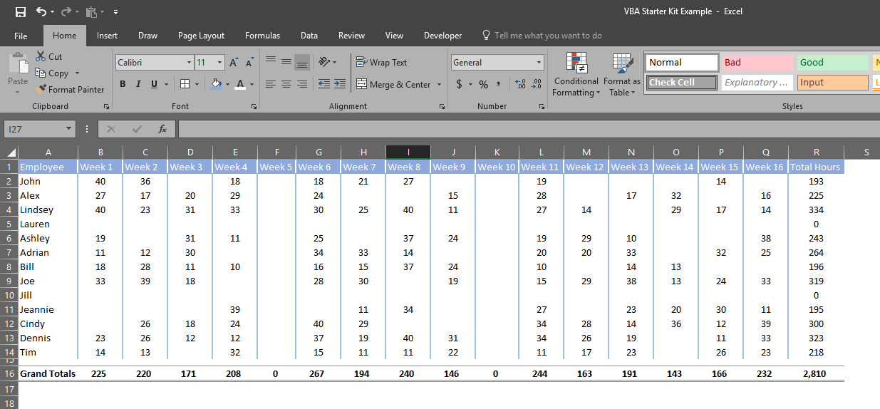
Being able to hide unnecessary rows and columns is great for making your data look clean and neat. No one likes all that whitespace, but hiding rows requires a lot of clicking or keyboard shortcuts.  Using a small bit of code, we can automate this process and save users some time. This is also a notable example of code you might write inside a sheet object rather than a module!

The Data:

The Code:

Sub Hide_Rows_and_Cols()
Dim i As Long
For i = 2 To 14
    If Cells(i, 18).Value = 0 Then
        Cells(i, 18).EntireRow.Hidden = True
    End If
Next i
For i = 2 To 18
    If Cells(16, i).Value = 0 Then
        Cells(16, i).EntireColumn.Hidden = True
    End If
Next i
End Sub

Sub Unhide()
Sheet3.Cells.EntireRow.Hidden = False
Sheet3.Cells.EntireColumn.Hidden = False
End Sub

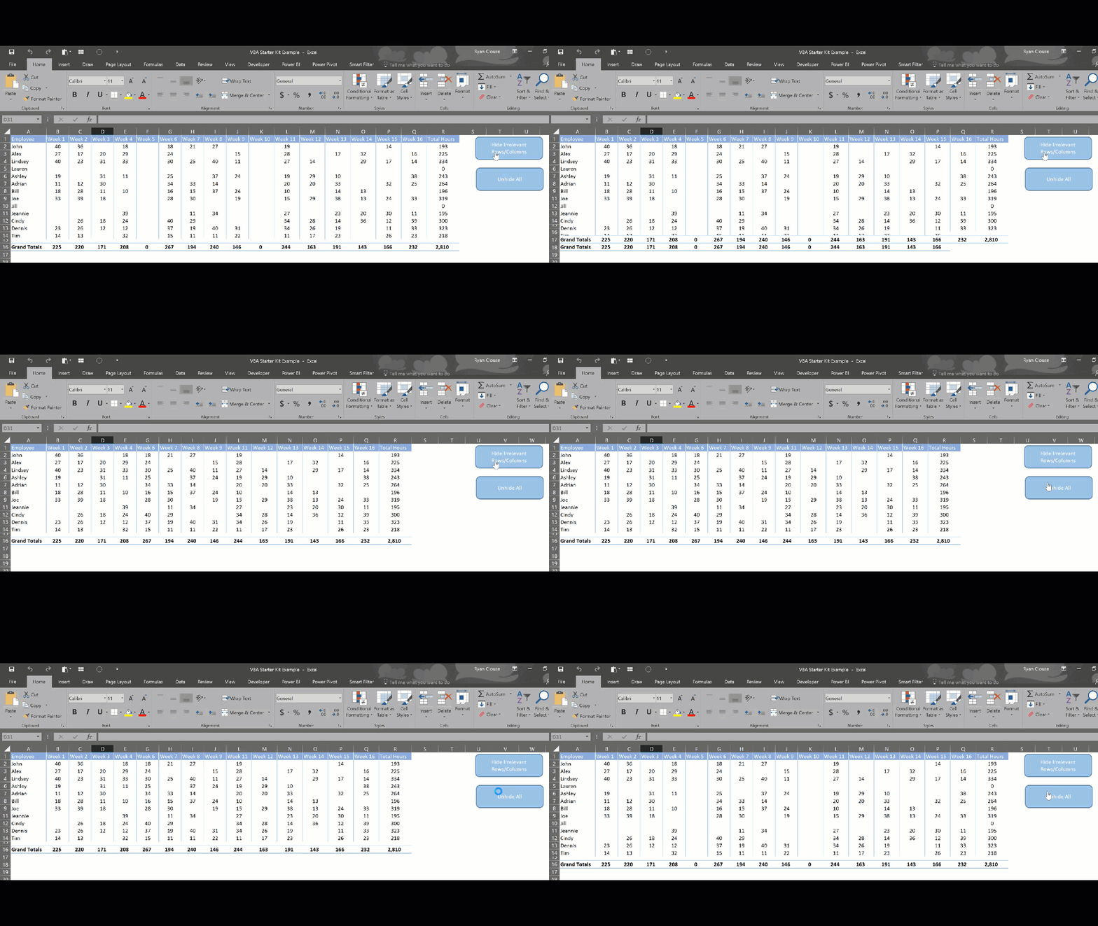
The Result:

VBA Hide Unhide Rows Columns

The Explanation:

So – what happened?  We created two subs at the Sheet3 level and attached each of them to a shape embedded in the worksheet. When the user clicks on these shapes, the sub is called and condenses the report to show only applicable information.


The “Unhide” sub simply sets all the rows and columns on sheet3 to visible.


The “Hide_Rows_and_Cols” sub is slightly more complex. It inspects the total column for rows that total zero. If the row total does equal zero, it hides the entire row from the spreadsheet.  The sub then does the same for each column total. I chose this example because, although it is simple, it demonstrates a “for loop”.


For loops are an essential concept to learn to write well performing and dynamic code and are present in every language. There are two ways to write for loops.  You can define the number of times the loop is to perform, as I did in my sub. You can also do a “for each” loop that will run for each occurrence of whatever you wish.  For example, you might want to do something for each cell within a range.  Let’s look at what my sub would have looked like had I chosen to go this route initially.

Sub Hide_Rows_and_Cols2()
Dim i As Long
Dim rowTotal As Range, colTotal As Range
Set rowTotal = Range("B16:Q16")
Set colTotal = Range("R2:R14")
For Each cell In rowTotal
    If cell.Value = 0 Then
        cell.EntireColumn.Hidden = True
    End If
Next
For Each cell In colTotal
    If cell.Value = 0 Then
        cell.EntireRow.Hidden = True
    End If
Next
End Sub

VBA Code Example – Run Code on Cell Change or Another Worksheet Event

In today’s “everything at the tip of your fingers” world, everyone wants to do more with less. Working with data in Excel is not exempt from this trend. Many executives (and non-executives) do not want to navigate filters, click through multiple tabs, copy/paste, etc. Being able to write code that can run as users interact with sheets is an incredibly important asset.


To accomplish this, we will use event handling. VBA has preset event names you can use to code around events. Here is a list of those events. It is important to note that this list is only for worksheet events. That means that the actions are all based on how a user interacts with a given worksheet. To perform one of these actions, you need to place a sub, titled as the event name, in the worksheet object you want to affect.

The Data:

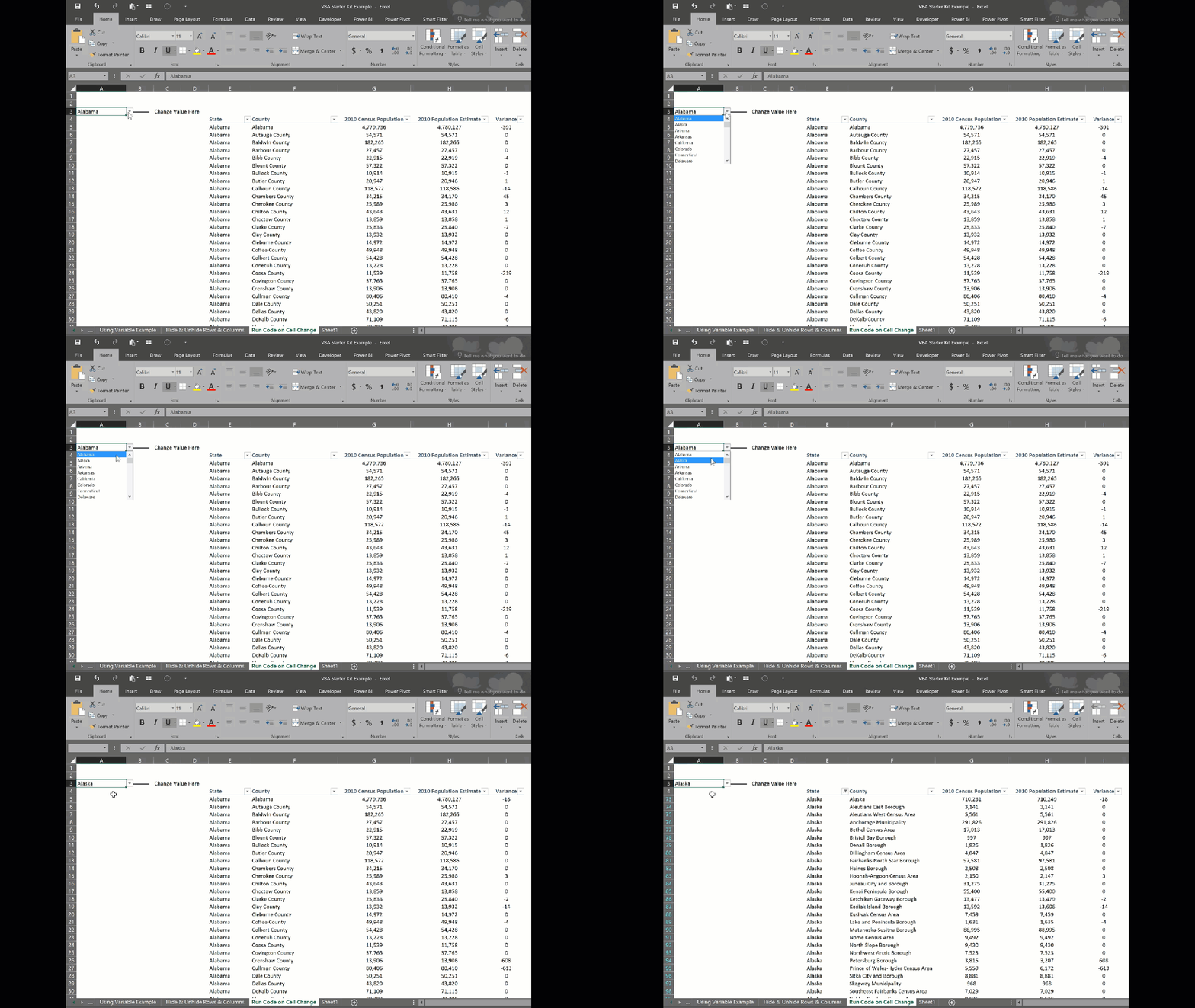
In this VBA code example, we have a list of states and counties with estimated population and census results and want to give the ability to filter results based on a separate dropdown.

The Code:

Private Sub Worksheet_Change(ByVal Target As Range)
Dim changeRange As Range
Set changeRange = Range("A3")
If Not Application.Intersect(changeRange, Range(Target.Address)) Is Nothing Then
    Range("populationData").AutoFilter Field:=1, _
        Criteria1:=changeRange.Value, _
        Operator:=xlFilterValues
End If
End Sub

The Result:

The Explanation:

The sub starts off with the line “Private Sub Worksheet_Change”.  The compiler for VBA recognizes this as an event handler and will trigger this sub when that specific even takes place.  Again, it’s import to note that this only affects the worksheet object in which you place the sub.


The next section of code is very important.  We set “changeRange” as a Range variable and assign it to the cell A3 on the worksheet.  Then, by using the Intersect function to check if the worksheet change happened in that cell, we can limit our code to run only when that cell value changes. Without this check, whatever code you place here will run anytime a worksheet change happens.  While that can be the desired effect, it certainly isn’t in this case.  


In case you’re wondering, the “populationData” range is a named range within my workbook. Naming ranges in your workbook makes referencing them within VBA very easy and I highly recommend it. The drawback is, if your dataset size changes, you need to make sure your named range resizes to accommodate or you could be missing some data in your data set.  If that’s the case, you’re better off dynamically setting your range with code (blog post coming soon on this!).  I usually use named ranges when it’s a single cell input I need to reference in my code or a row of column headers.  


Lastly, I want to remind you that you can run code when other events happen as well. Worksheet_Change is probably the easiest event handler to use and there is a ton of examples out on forums for you to use, but be sure to browse the event handler list I referenced early to determine what is best for your scenario.

VBA Code Example – Working with Strings in Excel VBA

Often, I’m using VBA to change data I’ve pulled from some data source. There are a lot of reasons one might do this. Perhaps the end user prefers a certain format, the data could be poorly formatted upon export, to compare the data, you must change it to match other data. The reasons are endless and, fortunately for us, VBA is a wonderful tool for working with and editing strings.

The Data:

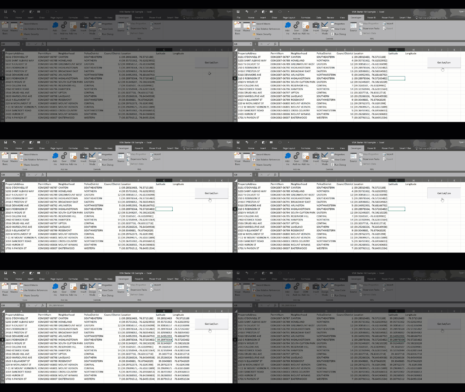
For this VBA code example, I’m using a small sample listing of housing permits. The sample includes a “Location” column which represent the latitude and longitude coordinates. If we want to get the latitude/longitude into separate columns from this, we need to read and edit the location string.

The Code:

Sub Get_Lat_Lon()
Dim loc As String
Dim sht As Worksheet
Set sht = Worksheets("Working With Strings")
For i = 2 To 19
    loc = sht.Cells(i, 6).Value
    sht.Cells(i, 7).Value = Mid(loc, 2, InStr(1, loc, ",") - 2)
    sht.Cells(i, 8).Value = Mid(loc, InStr(1, loc, ",") + 1, Len(loc) - InStr(1, loc, ",") - 1)
Next i
End Sub

The Result:

The Explanation:

Working with strings in VBA can look complicated at first glance, but it’s quite simple once you begin to think of strings as a sequence of numbers representing the position of each character. If your string is 10 characters long and the information you need is represented by characters 4,5,6 &7, then writing your code becomes about isolating those characters. Before I dive into what I did, let me first give a brief explanation of each VBA function I used.


  • Mid you might recognize this formula from Excel if you’re familiar with Excel’s text formulas. The mid formula allows you to return a given length of text from a string from a starting point you specify.
  • Instrif you’re completely new to VBA, this is probably something you’ve never seen.  The InStr function returns the numbered position of the first occurrence of a character within a string after a given starting point.
    • Example – InStr(1,”Apple:Orange”,”:”) would return the value 6 since the colon is the 6th character.
  • Lenthis is the simplest function as it returns the total number of characters within a string.


After examining the format of the location column, I could see that the two pieces I wanted were contained inside of parenthesis and separated by a comma. Knowing this, I could use the comma to determine the length of each of my strings I wanted to return.


For latitude, I needed only the first number so I started from the second position (skipping the parenthesis) and determined the length of my string by using the InStr function and subtracting 2 (2 because of the comma and the starting position of 2).


For longitude, I needed the second number. Therefore, I start at the comma using InStr function and adding 1 (adding 1 due to the space that separates. You could also have left this alone and used a Trim function). I determine the length by using the Len function to get the full length of the string and subtract the starting point and one additional character to remove the parenthesis.  


I hope at least one VBA code example is useful for you. If you want the working file I used for the examples, don’t forget to subscribe to my site for access to that file and all my other example files and free Excel templates! I’ll never share your information and won’t spam you with dozens of emails. If you have questions about the content, post in the comment section or shoot me an email at ryan.clouse@excelerator.solutions. I look forward to hearing from you!

Help-Desk