

09 Aug Using Excel Custom Views to Hide Columns & Rows
Howdee! The ability to hide columns in Excel (or rows) is not a topic that’s ground-breaking news by any means. It’s probably something you do on a regular basis. However, have you ever found yourself creating multiple views of the same report depending on the audience? Often, this requires a separate tab which is more work for you as an analyst, not to mention it increases the size of the file and resources required to update. Using Excel custom views can make this process smoother and can provide some nice interactivity to viewers of your report.
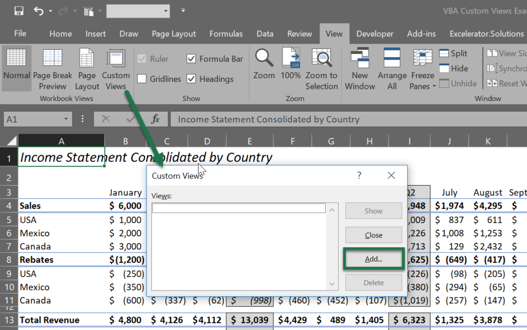
To get started, I’ll be working with a short month over month income statement that has subtotals by quarter. The example file looks like this to begin:

There is a lot of detail here that may or may not be necessary depending on the audience. It would likely be beneficial to allow the user to quickly switch between views of quarters only, no quarters, all detail, USA detail only, etc. You could write some macros that would hide columns/rows based on certain criteria (shameless plug: check out the VBA Starter Kit section for an example of this), but this could be unnecessarily complex in a real-world example. Therefore, creating custom views could be a much quicker approach.
Creating Excel Custom Views
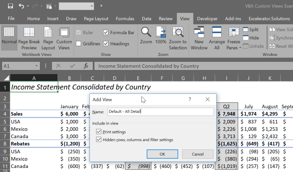
For those of you asking yourselves “I didn’t know about the Excel custom views feature?”, let’s first cover how to create a basic custom view in Excel. I like to create my first custom view as “Default”. This allows me to always get back to my full data view quickly. To do so, before you start organizing any views, click on “Custom Views” on the “View” ribbon, then click “Add”. In the next window, name the view whatever you like, I prefer “Default – All Detail”. Now click “OK” and your view is saved.
Next, start creating your first view by hiding applicable rows/columns. A little-known side note here, a shortcut to hide columns in Excel is ctrl + 0 and the shortcut to hide rows is ctrl + 9. It will hide whichever row/column is related to whatever selection you define. This saves a lot of time when creating these views. Once you’ve hidden your desired rows/columns and adjusted your zoom to something appropriate, then follow the same process as above to create a view of the current setup. In my example, I’ve hidden the quarters columns and increased the zoom to 115%. I saved it as “No Quarters – W/Detail”. We now have a basic view that will hide columns in Excel whenever we apply it. I have also created several other views to demo the different ways to apply custom views in Excel.
Three Ways to Apply Excel Custom Views
Use Custom Views Interface to Apply Views
The custom views interface already allows you apply views from it’s interface after you have created them. Simply click on “Custom Views” on the “Views” ribbon and you can double click any of the views you have created. Alternatively, you can click “Show” to apply the currently selected view. “Close” will close the custom views window. We have already covered “Add” and the last option “Delete” will delete the selected custom view.

This option is fine provided your user knows how to access it but there are a couple of approaches I find to be better.
Add Dropdown to Quick Access Tool Bar to Apply Views
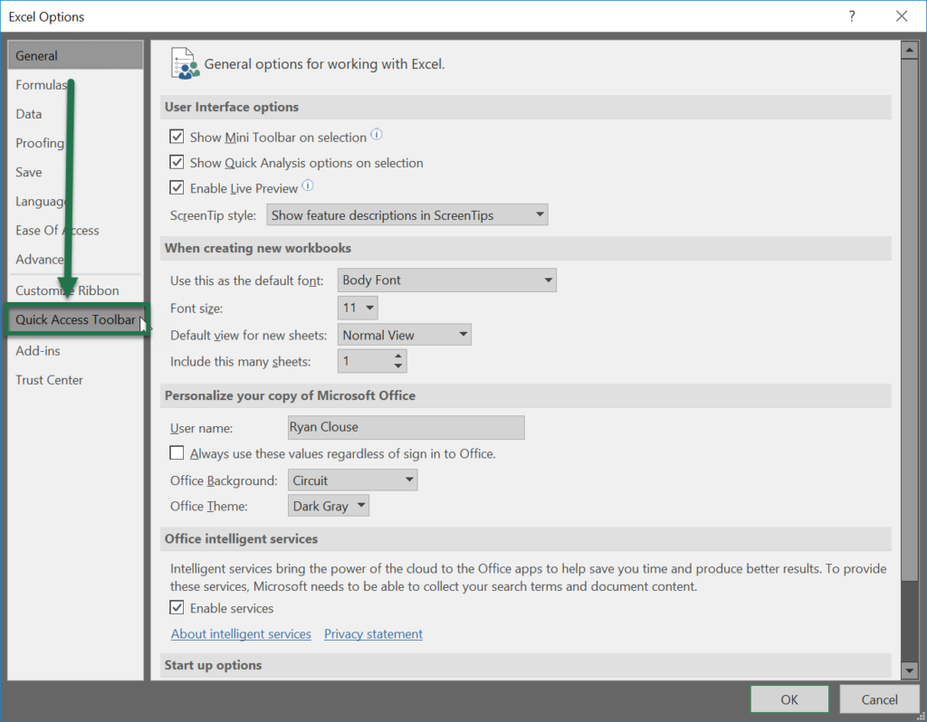
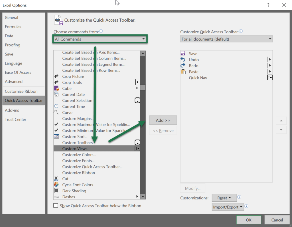
Another option is to add a dropdown to your quick-access tool bar that will allow you to select any of the available views in this workbook. To add this, go to “File” and select “Options” at the bottom of the pane on the left side of the application. This will open up the “Excel Options” window. Select the “Quick Access Toolbar” section. Also, you can get to this screen by right-clicking anywhere in the Excel ribbon and selecting “Customize Quick Access Toolbar”. Once here, change the dropdown under “Choose Commands From:” from Popular Commands to All Commands. The commands are listed alphabetically and you’re looking for “Custom Views”. Once selected, click “Add” to add it to the toolbar and then click OK in the bottom right.
Now that you’ve created the dropdown, you can select any of the views from it and they’ll be applied!

There are a few cons to mention with this approach. The quick access toolbar is only saved in the settings for you as a user. So, even though you’ve added the Excel custom views dropdown to your toolbar, others will likely have to be instructed to do so. Also, the toolbar will always be there, even if there are no custom views saved in the workbook. Not a huge deal, but may not be what you want. These issues are why I generally gravitate towards the final approach.
Apply Excel Custom Views Using VBA
“Using VBA” might intimidate you if you’ve never written a line of code in your life. Don’t let that scare you off though, this approach only requires a couple of simple lines of code to manage. Before we get started writing the code though, we need to set up our own custom dropdown. If this is new to you, read here to learn how to create dropdowns in Excel. We will put our dropdown on the tab whose view we want change.
I generally create my list on a separate tab called “Criteria” and hide that tab. It’s important the values in the dropdown match exactly to the names of your custom views. Secondly, the location of your dropdown matters. It is important to consider which rows/columns you’re hiding so you don’t hide the dropdown from your user. In this example, I’ve chosen to put the dropdown in cell A2 below the title of the spreadsheet so it is always visible regardless of zoom.
Now, press alt + F11 to open the VBA editor. Double click the sheet where your dropdown is located and, in the window that opens, place this code:
Private Sub Worksheet_Change(ByVal Target As Range)
Dim KeyCells As Range
Set KeyCells = Range("A2")

If Not Application.Intersect(KeyCells, Range(Target.Address)) Is Nothing Then
    ActiveWorkbook.CustomViews(Cells(2, 1).Value).Show
End If

End Sub
This code will trigger anytime the dropdown value is changed. Please note that you’ll need to change the references ‘Set KeyCells = Range(“A2”)’ and ‘ActiveWorkbook.CustomViews(Cells(2, 1).Value).Show’ to reference where you have your dropdown located. Now the end user can simply select form a dropdown embedded in the sheet to change the view of the data he/she is seeing. This is the best approach in my opinion as it does not require any additional knowledge from the end user regarding custom views.

Lastly, I would like to point out a quick limitation of using Excel custom views. If you have any tables in your workbook at all, you’ll need to convert them to ranges. Tables in a workbook will deactivate the custom views for that workbook. A strange limitation in my opinion, but definitely one that you should know about. Here is a useful link on troubleshooting custom views if you run into any issues.
I hope this article has demonstrated a great use for Excel custom views that you may not have known before. If you have other approaches to quickly changing the display of your worksheets I’d love to hear about them in the comments below!
Cheers,
R
No Comments