
11 Oct Getting the Most out of the Excel Sumif Function
Howdee! Going back to Excel’s early days, one of its primary uses has always been the aggregation of data. Being able to sum and count data on the fly in a spreadsheet was a revolutionary change to the workplace. Many years later, those formulas are often the backbone of Excel models and spreadsheets. Today, I want to cover off on one of these functions I’ve used heavily over the years; the Excel sumif function. This function, and its cousin sumifs, are incredibly useful when you need to aggregate data that meets certain conditions. They allow you to leave your data in its original state and perform filter your aggregations in formula. With introductions out of the way, let’s dive in!
Excel Sumif Function
Syntax: SUMIF( range, criteria, [sum_range] )
The Excel sumif function does exactly what its name implies. It sums data if some criteria is met. The “range” parameter is the range that will be evaluated against your criteria parameter. The criteria parameter is the criteria you’re wanting to be TRUE in order for the formula to sum it. Lastly, the “sum_range” parameter is an optional parameter that points to the range you’re wanting to aggregate. If you leave this input out, Excel will assume you want to evaluate the column in the “range” input against your criteria and sum that column.
An important note about the Excel sumif function is that it is limited to a single criteria. The sumifs Excel function (which we will cover in just a bit) allows for multiple criteria. Let’s take the sample data below as an example:
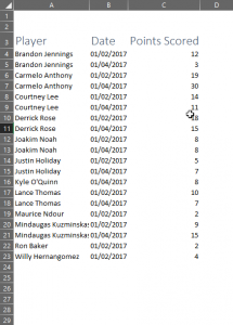
With this small dataset, a sumif is unnecessary but, for example’s sake, let’s say we need to show how many points were scored by Derrick Rose over this time frame. Stepping through the syntax above, our range would be the list of player’s names, the criteria would be “Derrick Rose” and the sum_range would be the points column.

Another important callout with the sumif formula is that you’ll want to make sure that the arrays are the same size. Other functions, like sumproduct, will throw an error if your input ranges are varied sizes. However, sumif will not. Thus, it is important to make sure up front that your inputs are the correct size. Trust me, this is an annoying error to track down later.
Sumifs Excel Function
Syntax: SUMIFS( sum_range, criteria_range1, criteria1, [criteria_range2, criteria2, … criteria_range_n, criteria_n] )
If you understood the sumif function, then the sumifs Excel function should be a piece of cake (mmmm cake!). The advantage of this formula is, as the s on the end indicates, you can have multiple criteria to evaluate against. Looking through the syntax, the first thing you might notice is that the sum range has moved to be the first input and it is no longer optional. You must first select your sum range and then your criteria range and, finally, your criteria to evaluate against. You can then repeat criteria range and criteria for that range as many time as necessary.
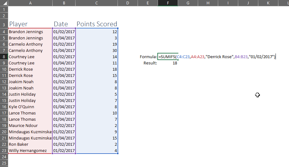
Continuing from our previous example, let’s assume you also want to limit the results of your sumif to only the January 2nd game. Our first input is now the points column, the criteria_range1 input is going to be our list of player names and the criteria1 will be “Derrick Rose”. However, we will also add the date column as a criteria_range2 input, and “01/02/2017” as the criteria2 input.
One of the wonderful things about the Excel sumifs formula is, unlike the sumif formula, it will throw an error if your criteria ranges are not the same size as your sum range. This is much more helpful for trouble shooting spreadsheets. For this reason alone, I recommend always using the sumifs formula over its brethren.
Quirks of the Excel Sumifs Function
While these two formulas are somewhat self-explanatory, my primary reason for writing this article is to shed some light on a couple of quirks regarding the use of these functions.
Sorting Excel Sumif Formulas
Many times, you might have your sumifs formula as part of a larger dataset and you or another user might end up filtering that data. Depending on the syntax of your formula, this can actually cause errors in your results. This generally happens when your formula is linked to another worksheet or workbook. However, it can happen even if data is on the same tab!
The error comes when your criteria is on the same worksheet as the formula, but you still reference the worksheet. That may sound strange so let’s examine the following example:
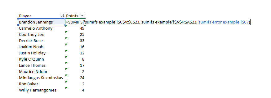
In the formula, you can see that I’ve referenced data on another tab for my sum range and criteria range. However, when you navigate back to the tab to select the criteria to evaluate against, it puts that tabs name in front of the criteria input. You wouldn’t think this would be a big deal but, if you sort the data, your inputs can unarranged themselves. Let’s sort the list and take a look again:

Wow! If I handed this off to someone and they sorted my formulas, they may or may not catch that this formula has an error! I think this bug is on Microsoft’s radar and I would assume to see it resolved soon but it’s definitely something you should be on the lookout for if you’re working cross worksheet/workbook with your Excel sumif formulas.
Returning Greater Than/Less Than with Sumif Formulas
When I was first starting to do data analysis in Excel, nothing frustrated me more than having to evaluate sumif(s) and countif(s) formulas for greater than/less than criteria. For some reason, this was one of the hardest quirks for me to remember about Excel sumif formulas. When working with literal dates in a sumif formula, the date and greater than/less than (including the equals symbol if necessary) should be treated as a literal string.
What does that mean? In Layman’s terms, it means your text should be wrapped in quotation marks. So if you’re wanting to sum rows where a column date is greater than or equal to January 1st, 2017, you would have a formula that looks like this:
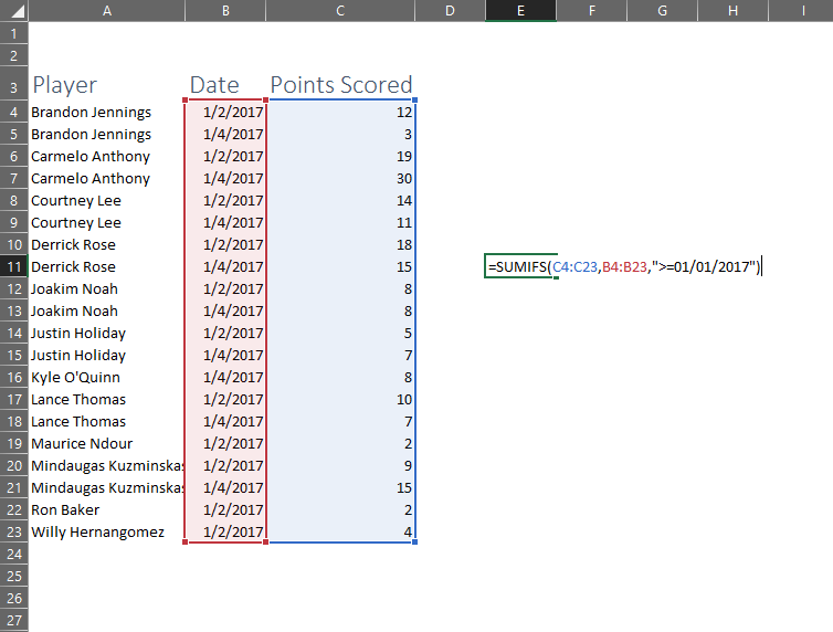
That’s pretty easy to understand when you’re typing the date into the formula itself. However, what if you want the date to be determined by what a user types into a cell? You’ll need to concatenate the string inside the formula with the cell. Again this may not make a ton of sense when read, so let’s take a look at an example:
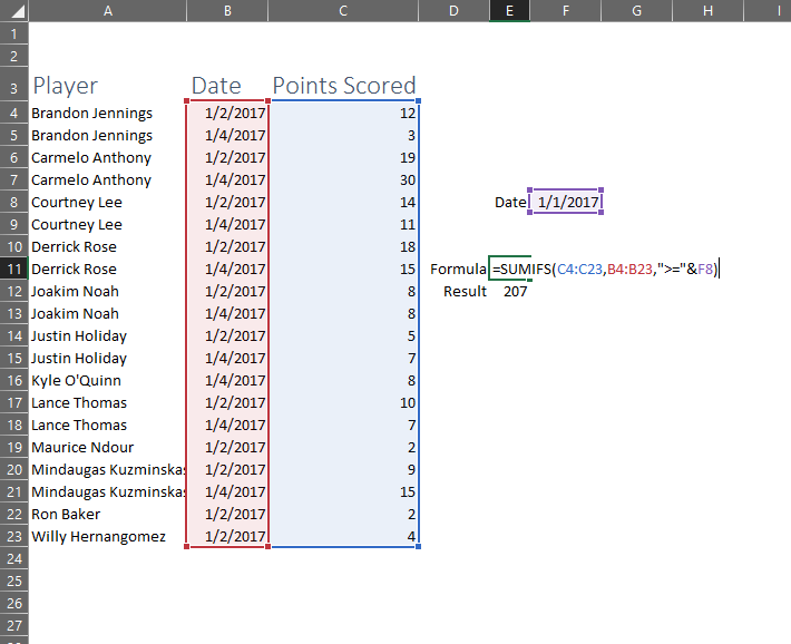
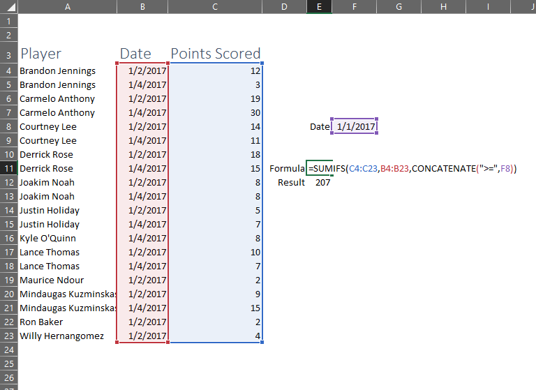
The result of this is still the same, but the formula input is very different. Using the ampersand, we can join together the cell input and our symbol to make this formula a little more dynamic (Hint: you can use two cell inputs and allow the user to select the symbol and criteria as well). Just to be thorough and show that it is expecting a literal string, using the concatenate formula in place of the ampersand returns the same result:
I hope you’ve found this introduction to using the Excel sumif and sumifs formulas useful. If you have any questions or have any other “quirks” to add please drop them in the comments below. As always, you can get the workbook I used in my examples in the example files section of my site if you’re a free member.
Cheers!
R
No Comments