
14 Aug Top 5 Excel Vlookup Tips & Tricks
Howdee! The Excel vlookup function is one of the most common job requirements listed for any position that will require the applicant to use Microsoft Excel frequently. However, many folks aren’t utilizing the vlookup function to its maximum. There are several uses of the Excel vlookup function that you might not know about, I am going to cover off on five of them today.
One – Basic Excel Vlookup
For those of you that may not know even the basics of a vlookup function, let’s cover that first (click here if you’re a visual learner). The Excel vlookup formula will look for a value you specify in the left-most column of the table you define, and return a value, in that same row, from a column you specify. Excel can either return an exact match (most common use) or an approximate match. Let’s examine the syntax below and step through the inputs:
=VLOOKUP(lookup_value,table_array,col_index_num,range_lookup) ***custom CSS to border and back
- lookup_value | this is the value you’re attempting to lookup in the left-most column of a table, and return some value in that row when it matches.
- table_array | this is the table you select where the left-most column contains the “lookup_value” you used for the first input.
- col_index_num | this is the number of the column where the data you’re attempting to return lives. For example, let’s say you have three columns “name”, “address”, & “city” and you’re vlookup is trying to return “city” from lookup_value “name”. The col_index would be 3 since it is the third column in the table.
- It’s important to note that if your lookup_value was “address” the col_index would be 2 since it is the number of cols based on the left-most column you select in the table_array input.
- range_lookup | this is either “TRUE”, for an approximate match, or “FALSE”, for an exact match. If you use “TRUE” then your data will need to be sorted in ascending order on the left-most column in your selected table_array
Two – Find Missing or Invalid Data
When performing data analysis, ensuring data accuracy is incredibly important. Sometimes however, this can be easier said than done. Using the Excel vlookup function can help you identify missing pieces of data and data that doesn’t match between data-sets. Let’s look at this simple data for an example.
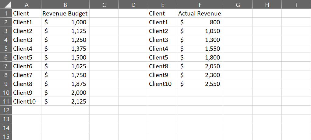
You can easily see that the data-set on the right is missing two values. Now, in this simple example, It is easy to identify what is missing, but if there are dozens, hundreds, or even thousands of data points, it becomes much more difficult. If you use the Excel vlookup formula and ensure you are using “FALSE” for the “range_lookup” input, you can easily identify what’s missing. Let’s take a look at this data-set again, but I’ve used a vlookup formula to show which values are missing from the second data-set.
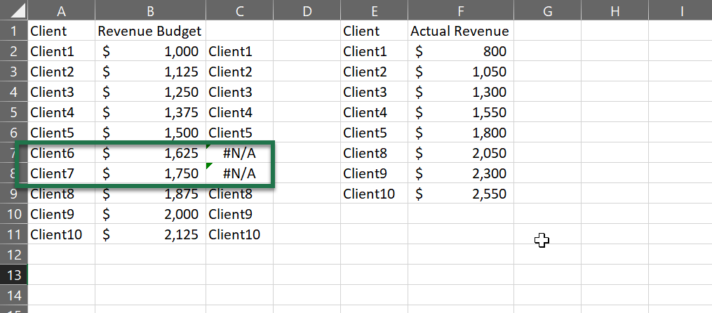
You can easily see that the vlookup returns #N/A when the values don’t exist in the opposite list. On larger data-sets, you could then filter to rows where the #N/A appears and investigate.
This solution is also very useful to ensure that data matches between systems. Let’s say you have to disparate systems and you need to marry data from both. In one system, names are preferred names, and, in the other, you have legal names. Using a vlookup to see where values don’t exist between datasets can help you quickly identify which pieces of data to change. This is my favorite use of the Excel vlookup formula as it saves me huge amount of times when comparing disparate datasets.
Three – Make Excel Vlookup “Unbreakable”
Often, vlookup formulas power templates that other colleagues are using. These colleagues may or may not be familiar with this formula and it’s something you should consider when building the formula. Using a few tips to help ensure the user won’t “break” the formula can help prevent a lot of questions and frustrating errors.
Firstly, you should always use absolute references when applicable. Absolute references ensure that, if uses drag or copy/paste functions to the left or right, they will still reference the correct data. I typically use an absolute column/relative row (exe: $A1) for the lookup value input, and use an absolute column and absolute row (exe: $A$1) for my table array. On occasion, I’ll use an absolute row, relative column reference (exe: A$1) for my column index input. This allows me to utilize one row for my column index inputs and drag vlookups across. This is especially useful when doing vlookups to return monthly data as shown below.
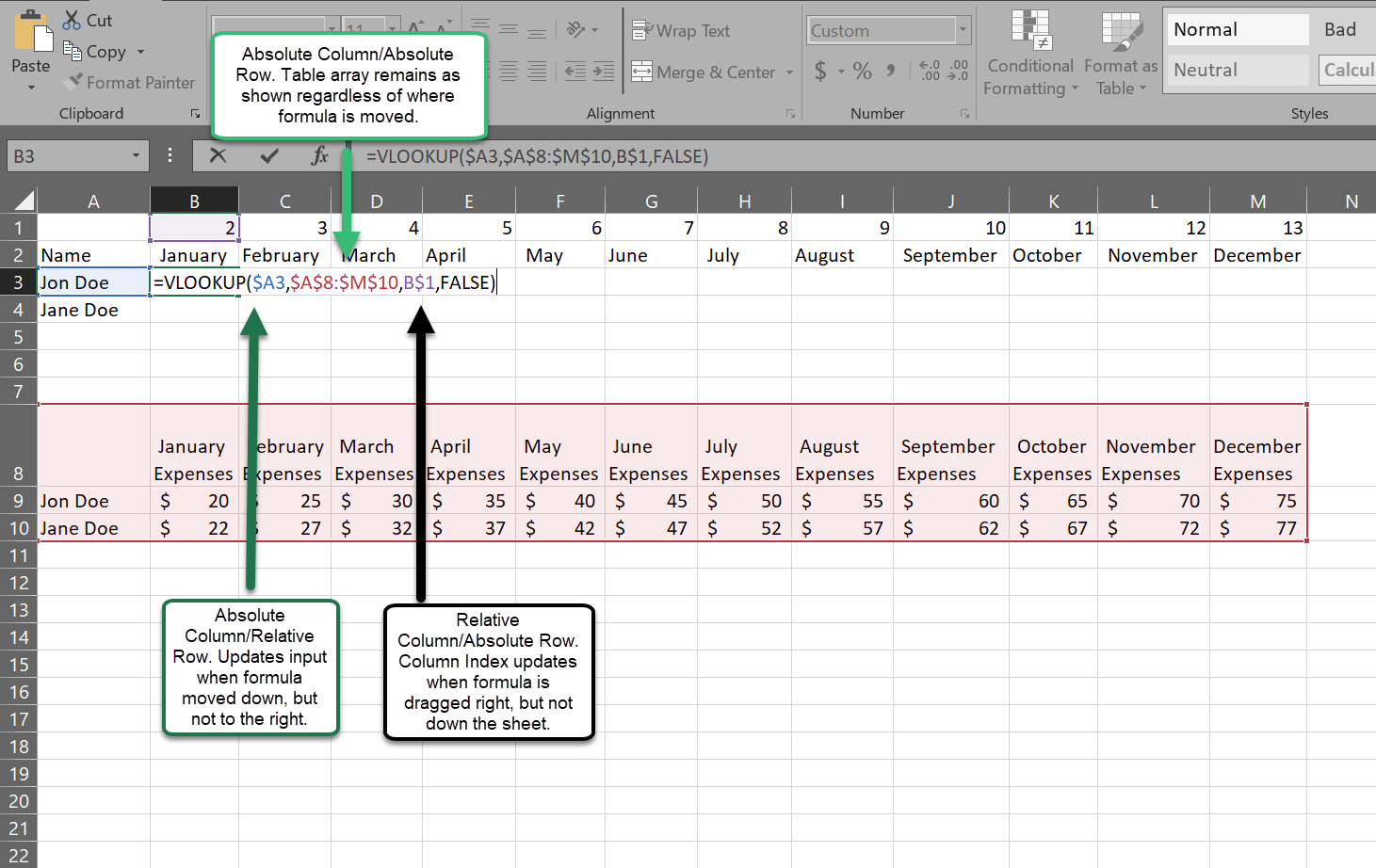
To go a little further, you can make the column index even more dynamic by using the match formula for that input. Let’s examine the match formula syntax.
=MATCH(lookup_value,lookup_array,match_type)
The “lookup_value” & “lookup_array” inputs are very similar to the lookup value and table array inputs for the vlookup formula and behave the same way. The “match_type” input is either a 1 (less than),0 (exact match), or -1 (greater than). If you use the less than match type, you must ensure your data is in ascending order. Likewise, if you use the greater than match type, it should be in descending order.
The match function returns a number equal to the matches position in your array. Let’s look at the previous example with a match function for the column index input.
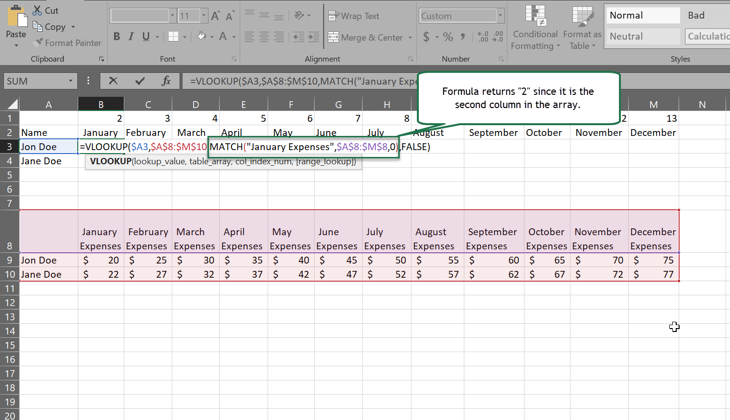
You might think this is a lot of extra work for the same result, but this is very useful if columns in a dataset may be in random orders, or if the user may insert a column. Please note, it’s very important that your lookup array for match is the same size as your table array for your vlookup so the column number returned is accurate. Also note that, if there are multiple column headers with the same exact heading, the match formula will return the first if they’re not adjacent, but will return the last if they are adjacent.
Four – Vlookup Replace Nested If Statement
An Excel vlookup function can be used to evaluate a less than and greater than criteria. This is the most common approach for using the “TRUE” range lookup type. Let’s assume we have a list of orders and we’ve promised a 20% discount on the first 5, a 10% discount on the next 5, a 7.5% discount on the next 5 orders, and a 5% discount on the next 5. You could use several nested if statements like this.
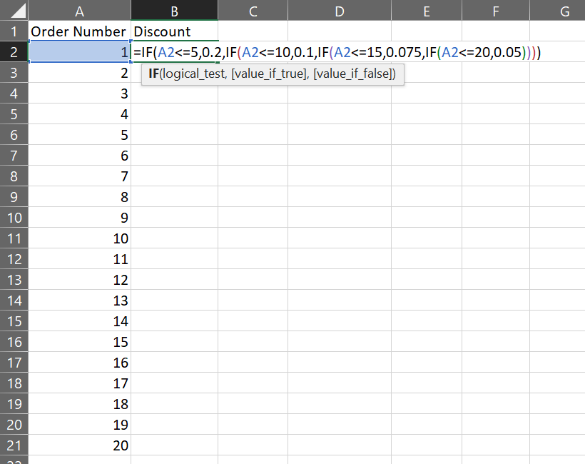
This would achieve the desired result, but is difficult for others to follow and, if the discounts needed to be changed, it would require major adjustments to the formula. Another approach would be to create a discount table and use an Excel vlookup formula (with “TRUE” range lookup input) to evaluate it. As you can see below, this returns the desired result and an update would only require an update to the lookup table, rather than a change to the formula itself.
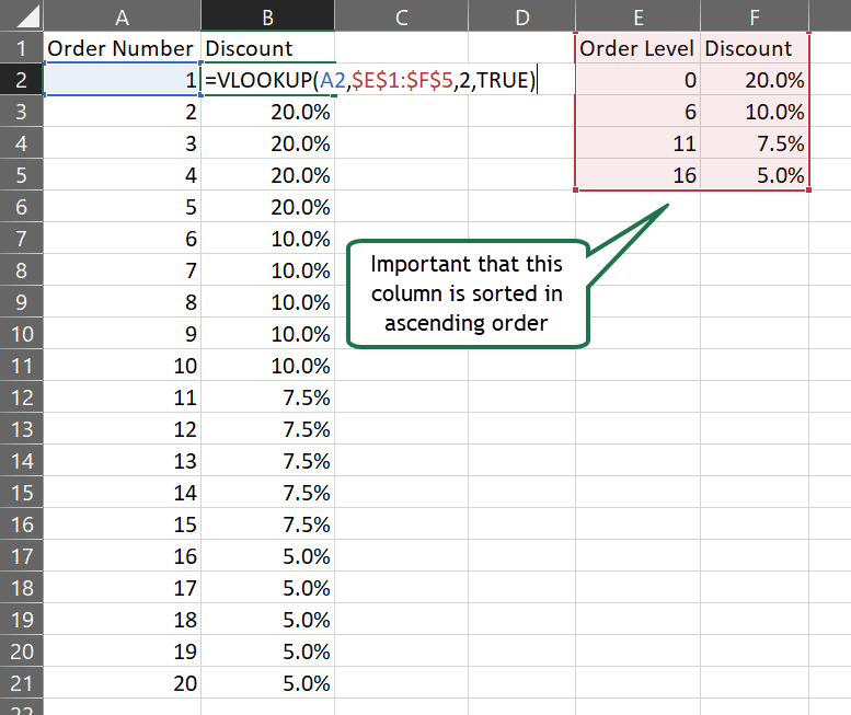
It’s very important to note that order matters when using the “TRUE” range lookup input. Ascending order will act as a “less than” qualifier, while a descending sort would act as a “greater than” qualifier.
Five – Use Tables & Named Ranges When Applicable
Using tables and named ranges can help with readability of your formula, especially if you’re handing off to someone who has never seen your data before. The formula will include references to table and column names in the formula like the below.
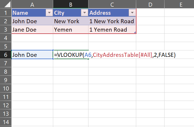
Even if you know nothing about this data, you can quickly see that this vlookup is returning information from a table named “CityAddressTable” and you’re able to investigate. This also has the added benefit of referencing the entire table. That means, as you add rows of data to this table, you don’t have to worry about adjusting the size of the table array in your vlookup formula. It is always referencing the entire table and thus all the rows and columns. Combining this tip with some of the other tips I’ve referenced above can really help take your Excel vlookup formula skills to the next level.
If you have questions or suggestions, please drop them in the comments below.
Cheers,
R


No Comments